
ARIMA Model with EM price data
Here is a simple example of an ARIMA model with pricing data. This is just an example to show the basic code used for ARIMA. Statistical tests in order to choose the appropriate model/lags are not included.
import os
os.chdir(r”C:\Users\haderer\Documents\python”)
cwd= os.getcwd()
print(“Current working directory is:”, cwd)
import numpy as np
import sys
np.set_printoptions(threshold=sys.maxsize)
import pandas as pd
from matplotlib import pyplot as plt
from statsmodels.tsa.stattools import adfuller
from statsmodels.tsa.seasonal import seasonal_decompose
from statsmodels.tsa.arima_model import ARIMA
from pandas.plotting import register_matplotlib_converters
register_matplotlib_converters()
df = pd.read_csv(‘msciemret.csv’, parse_dates=[‘Date’])
df = df.replace(‘,’,”, regex=True)
df[‘Price’] = df[‘Price’].astype(float)
print(df[‘Price’].std())
df[‘Date’]= pd.to_datetime(df[‘Date’], format=’%b %y’)
df.info()
df = df.set_index(‘Date’)
df.sort_values(by=[‘Date’], inplace=True)
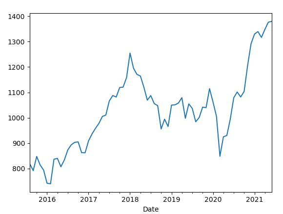
df[‘Price’].plot()
df_log = np.log(df[‘Price’])
plt.figure(2)
plt.plot(df_log)
plt.show()

df_log_shift = df_log – df_log.shift()
df_log_shift.dropna(inplace=True)
decomposition = seasonal_decompose(df_log)
model = ARIMA(df_log, order=(2,1,2))
results = model.fit(disp=-1)
plt.figure(3)
plt.plot(df_log_shift)
plt.plot(results.fittedvalues, color=’red’)
predictions_ARIMA_diff = pd.Series(results.fittedvalues, copy=True)
predictions_ARIMA_diff_cumsum = predictions_ARIMA_diff.cumsum()
predictions_ARIMA_log = pd.Series(df_log[0], index=df_log.index)
predictions_ARIMA_log = predictions_ARIMA_log.add(predictions_ARIMA_diff_cumsum, fill_value=0)
predictions_ARIMA = np.exp(predictions_ARIMA_log)
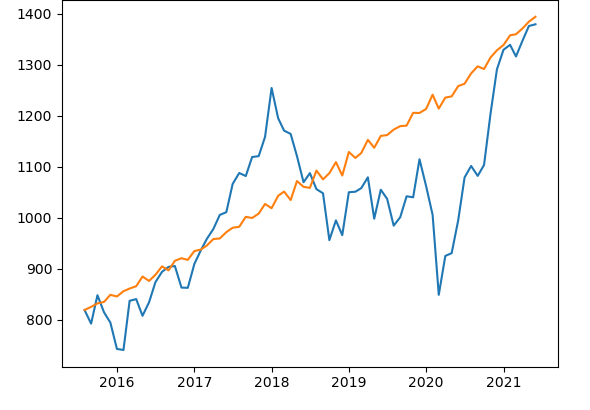
plt.figure(4)
plt.plot(df[‘Price’])
plt.plot(predictions_ARIMA)
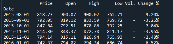
with pd.option_context(‘display.max_rows’, None, ‘display.max_columns’, None):
print(df)
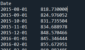
with pd.option_context(‘display.max_rows’, None, ‘display.max_columns’, None):
print(predictions_ARIMA)
RESULT:
s = predictions_ARIMA
df2=s.to_frame()
print(df2.head())
column_1 = df[‘Price’]
column_2 =df2.iloc[:,0]
correlation = column_1.corr(column_2)
print(correlation)
print(column_2)
print(column_2.describe())
print(correlation)
RESULT: 0.7501976605578393